It’s been a while since my last post, and my archive of unpublished projects has been piling up. It’s high time for a figurative sweep of the attic! As I went through this archive, I was pleasantly surprised by the number of cool projects I completely forgot about, and it was great to see that so many of them remain relevant and interesting today (at least, I hope so!). I originally wrote the code for this particular project years ago, and although I thought I left it in great shape, I also got a harsh reminder that code rots, and it did take non-zero effort to get it running again. But I did, so among the old results below are some brand new ones. After spending practically all of my time with AI for so long, it’s a refreshing change of pace to revisit some of the “classic” techniques we used to employ “in the old days”. This post describes such a technique. So, without further ado, let’s dive in!

A few years ago, after my child was born, I found myself constantly watching him sleep to check that he’s well. And when I wasn’t physically watching him, I was glued to the baby monitor. Unfortunately, since normal human breathing is so subtle, it was incredibly difficult to determine whether he was breathing, be it in real life or on the screen. To demonstrate the challenge, here’s a video example (it might look like a still photo, but I assure you it’s a video):

I had a weird thought - could I somehow amplify the motion in the camera to make it easier to discern that he is actually moving? It turned out that an extremely simple way (and basically the first thing that I tried) just works. No dataset, no training, just basic signal processing!

Update: As it turns out, in this project I rediscovered (a small part of) the amazing work Eulerian Video Magnification for Revealing Subtle Changes in the World, almost a decade after this seminal paper was published! In fact, this 2012 work by Hao-Yu Wu, Michael Rubinstein, Eugene Shih, John Guttag, Fredo Durand, and William Freeman recently won SIGGRAPH’s 2023 Test-of-Time Award, so if you are interested in the ideas from this post, I strongly recommend reading their much deeper paper.

The core observation was that the breathing motion that I wanted to amplify is periodic. What happens if we found the period and increased its amplitude? Specifically, what if we treat each pixel location (per color channel) as a 1-D signal in the time domain, find the strongest amplitude for all pixels, and amplified that? The following simplified code snippet illustrates this idea:

def amplify_max_freq(video, amp = 100):
  x = np.fft.fft(video, axis=0)  # f, h, w, c
  avg = np.abs(x).sum(axis=(1, 2, 3))
  mag = np.ones(x.shape[0])
  freq = np.argmax(avg[1:]) + 1  # Disallow the 0 frequency.
  mag[freq] = amp
  x *= mag[:, None, None, None]
  return np.fft.ifft(x, axis=0)

And that’s basically it! Here’s the result compared to the original video:

Success!

In this case, the video had 264 frames at 30 fps ($\frac{264}{30 \times 60} = 0.147$ minutes), and the strongest frequency was 8, which corresponds to $\frac{8}{0.147} = 54.5$ bpm, which I guess makes sense.

Notice that in the snippet above we just disallow the 0 frequency, but we could limit the frequency range further (e.g. to the 30-60 Hz range, which is a baby’s normal breathing rate).

It’s pretty remarkable that the spatial motion seems amplified, although (with the exception of finding the strongest frequency) all the processing happens only in the time domain, independently for each pixel!

Unfortunately, while the breathing is clearly magnified in the above video, the entirety of the video is noticeably noisier. Let’s deal with that. Our observation here is that while many pixels became noisy, in the area affected by the breathing the effect is much more dense. Our strategy then will be to modulate our motion magnification for each given pixel based on how affected the area surrounding the pixel is. First we’ll calculate the difference between the original video and the amplified video, and gaussian blur it across both spacial dimensions and across the channel dimension:

def gaussian_filter_nd(a, axes, sigma):
  for axis in axes:
    a = scipy.ndimage.gaussian_filter1d(a, sigma, axis)
  return a

blurred_diff = gaussian_filter_nd(amplified_video - base_video, axes=(1, 2, 3), sigma=30)

Next we’d like to almost zero out areas where blurred_diff is low, and only keep areas very close to 1 (and also made this 1-dimensional by summing across the channels dimension):

sharpened_diff = (blurred_diff ** 20).sum(3)

Now we’ll smear out the remaining values to their neighborhoods:

smeared_diff = gaussian_filter_nd(sharpened_diff, axes=(0, 1, 2), sigma=10)

Finally we’ll normalize smeared_diff and interpolate between the original video and the amplified video:

alpha = (smeared_diff - smeared_diff.min()) / (smeared_diff.max() - smeared_diff.min())
cleaned_video = base_video * (1 - alpha[..., None]) + amplified_video * alpha[..., None]

Here we see, from left to right, blurred_diff, sharpened_diff, and smeared_diff (the rightmost video shows overlays alpha on base_video for easy reference):

And here finally we have the full denoised result:

Yesa!

New Results!

Ok, so I said I got the code to work again - what could I test it on? One of the examples I tested a few years back was trying to amplify the motion of a person (myself) standing still. I decided to recreated that, so I took a short video of myself, trying as hard as possible to not move, and ran the code above on it (without the denoising part). Here’s the result:

Magic in just a few lines of code!

BTW - as part of getting the cobwebs off the code, I decided to use python-fire - it’s a super cool small library! Recommend to check it out.

Subtler Motion Amplification

We were able to amplify some motion, but can amplify even subtler movements?

Up to now, we’ve amplified the time-wise frequencies, entirely ignoring spacial relations between the pixels. Well here’s an interesting idea - what if decompose the high and low spatial frequencies of the video, apply our method only on the lower frequencies, and then recompose?

A simple way to get the lower spatial frequencies is to build a laplacian pyramid. This quick writeup has a great illustration of the related concepts of a Laplacian pyramid and a Gaussian pyramid. Basically, a Gaussian pyramid is obtained by repeatedly blurring and down-scaling an image (or a video in our case) and a Laplacian pyramid is the set of differences between consecutive elements of the Gaussian pyramid (the last one taken as-is):

downscale = lambda a: a[:, ::2, ::2]
upscale = lambda a: a.repeat(2, axis=1).repeat(2, axis=2)

def gaussian_pyramid(a, sigmas):
    res = [a]
    for sigma in sigmas:
        a = downscale(gaussian_filter_nd(a, axes=(1, 2), sigma=sigma))
        res.append(a)
    return res

def laplace_pyramid(a, sigmas):
    gp = list(reversed(gaussian_pyramid(a, sigmas)))
    res = [gp[0]]
    for i1, i2 in zip(gp[:-1], gp[1:]):
        res.append(i2 - upscale_vid(i1))
    return list(reversed(res))

Here’s the Laplacian pyramid (with 4 levels, all $\sigma$s=10) of my video:

Now let’s apply our amplification method on just the lowest element of the pyramid. Here is the graph showing the magnitude of the frequencies:

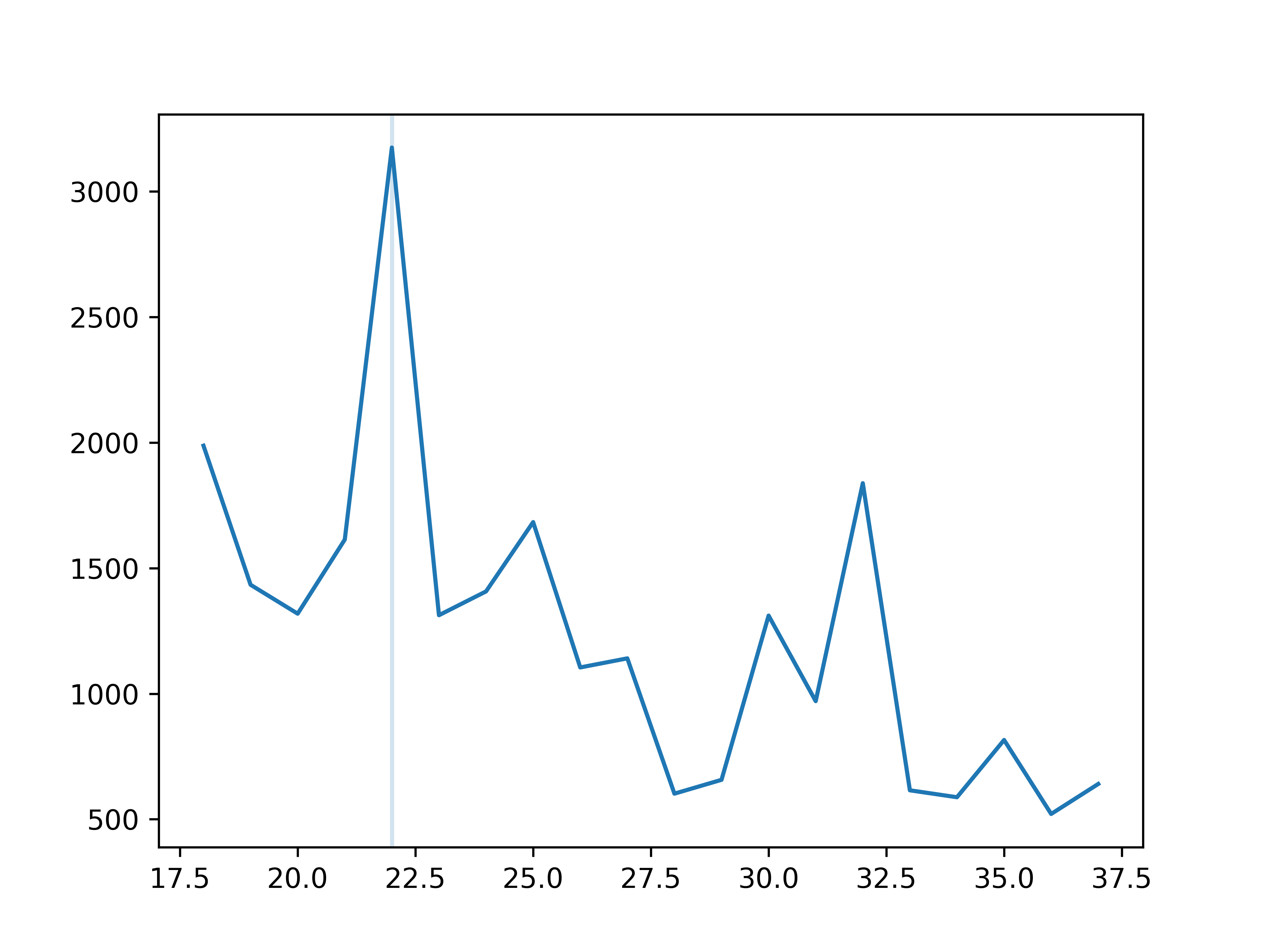
Frequency 22 (corresponding to 69 bpm) is the strongest. Could this be detecting my pulse?

Magnifying, with our favorite code piece above, just the lowest element of the pyramid and recomposing the video, here’s the result:

Could this actually be detecting my pulse??? I admit that while that is possible, I’m not sure - 69 bpm seems somewhat high, and I should have calibrated this measurement and actually measured my pulse to make sure. While I didn’t have a simple means to measure my own heart rate, I did plan to repeat this experiment after I do a bunch of high-intensity exercise and see whether I can at least measure a meaningfully higher rate, but I’ll leave that for a future update :)

Thanks for reading - hope you enjoyed reading this post as much as I enjoyed writing it!