A couple of years ago I was very interested in visualizing objects of more than three dimensions. I reasoned that if I stared at such objects for long enough time, I was bound to get a good intuition on how they look.

But how can one see objects of more than three spatial dimensions?

Our goal in this post will be to render an object residing in a coordinate system of arbitrary dimensions on a 2D computer screen. We will try to do this in such a way as to lose as little information as possible on the structure of the object, while maintaining its 2D description as simple as possible (so that indeed, we will get some form of intuition on the shape of the object).

The 4D Cube

Before we begin with the actual rendering process, lets explore some properties of the 4D cube. Lets start with the obvious:

• A 0D cube is simply a point.
• A 1D cube is a line segment. It has 1 * 2 = 2 faces each consisting of a 0D cube.
• A 2D cube is a square. It has 2 * 2 = 4 faces each consisting of a 1D cube.
• A 3D cube is, well, a cube (I hope that the repeated use of the word cube for two slightly different meanings does not confuse you). It has 3 * 2 = 6 faces each consisting of a 2D cube.
• Finally a 4D cube has 4 * 2 = 8 faces, each consisting of a 3D cube.

Here is a list of some interesting figures about the 4D cube. Can you figure out why they are correct? Can you generalize them to higher dimensions?

These values can be generated by my program, which is described below.

4D Cube Properties

• Number of edges: 32
• Number of facets: 8
• Facets per edge: 3
• Edges per facet: 12

3D Cube Properties (for comparison)

• Number of edges: 12
• Number of facets: 6
• Facets per edge: 2
• Edges per facet: 4

Dimensionality Reductions

I will now present several methods for encoding an N-dimensional object in (N-1)-dimensional space. Call such an encoding a 1-reduction. It will then be possible to encode any object on a 2D screen, by repeated applications of 1-reductions.

Let’s start by considering a very simple special case. Let’s say that our N-D (N-dimensional) object is actually an (N-1)-D object residing in N-D space. An example of this is an object with a constant coordinate. More complex examples exist (the object may not have any constant coordinate, but after applying some rotations, one of the coordinates may become fixed).

A basic 1-reduction can then consist of simply dropping the extra coordinate.

This may seem trivial, but I have a point here – when considering an inanimate object one of the coordinates is always fixed – that of the time!

Our first approach will then be trading a spatial dimension for a time dimension. I.e. encoding the Nth coordinate of an inanimate object by some form of animation.

A simple such encoding consists of slicing the N-D object. Consider the 3D case. If we denote the coordinate system of the object by x, y and z and the time coordinate by t, then we can select only points with a constant z coordinate equal to t. We would then get an animated 2D object representing our 3D object.

A key feature of this 1-reduction method is that no structural information about the object is lost by this encoding. Lets define this formally:

Definition - A 1-reduction of an object is called lossless if it can be reversed uniquely.

Using this definition, we can say that the method of animated-slices proposed above is lossless. Note that animated-slices is obviously not the only lossless encoding (can you think of others? 8-) ).

We will now restrict our discussion to smooth and bounded objects.

Definition – an object is called smooth if it can be approximated well by discrete boxes.

Definition – an object is called bounded if there exists a cube of finite sides that contains the object.

Cubes, spheres and rings are examples of smooth and bounded objects.

The smoothness of an object allows us to encode it using discrete samples. For example, when we display an animated slice of a 3D object on a computer screen, the animation consists of discrete frames each consisting of discrete pixels. A smooth object will be represented faithfully with such a discrete representation. More formally, lets define:

Definition – A 1-reduction is called casi-lossless if it can be reversed, and the difference between the inversion result and the original object is small.

So, encoding a smooth object as a sequence of frames is casi-lossless.

The advantage of considering only smooth and bounded objects is that we can encode two spatial coordinates on the same axis.

Lets start by demonstrating this with the simple case of a 3D cube (we will get to 4D cubes shortly!). This encoding is depicted here:

The image shows 2D slices of the 3D cube.

Note that the encoding is indeed casi-lossless: the entire structure of the cube can be reconstructed uniquely from the slices (again, neglecting small differences due to the fact samples are discrete).

Note that employing this method on a 4D object, instead of on a 3D one, results in 3D slices instead of the 2D ones. We can then apply another casi-lossless 1-reduction to the 3D slices, and get a casi-lossless 2-reduction from four dimensions to two dimensions (I leave to the reader to formulate the definition of a casi-lossless 2-reduction).

Projection

The method above, generalized slightly, is the most important 1-reduction method - the Projection. Projecting an object consists of simply ignoring one of its coordinates. It is actually simpler than what we discussed above – instead of converting one dimension to another (i.e. z-coordinate to t-coordinate) we simply ignore one of the coordinates.

This method by itself is obviously not lossless (it is not even casi-lossless). This means that there are many different N-D scenes that result in the same (N-1)-D projection. The method does work on a much larger scale of objects though, and this is the method we shall employ.

A projection of the rotated 3D cube is depicted here:

Note that unlike the slices version above, there is no way to tell whether this is actually a cube!

Can you visualize other 3D objects that would have this exact same projection?

A different rotation, like this one, might look more like a cube, but note that there are objects very different from cubes that would have exactly this projection:

Can you picture one?

Using Color

After projecting an object we can try to rescue some of the information lost by encoding it in the color channel.

In the picture below I encoded the same 3D cube as above, but this time the color of the object represents the depth at the pixel. The brighter the color, the closer the object:

Using the color channel thus does not make the encoding lossless. There is still no way to tell whether the shape above is that of a cube. It does considerably reduce the set of possible source-objects for the encoding though.

The main advantage of the projection method is that our brain is used to reversing projections. When you close one of your eyes, your brain receives a completely flat two-dimensional image. Even with both eyes open, you do not see a true three-dimensional image. You merely see two 2D images. Two projections of the 3D space in front of you!

Your brain does a great job at guessing the real 3D structure of objects by their 2D projections (it tries to calculate the most probable inverse of the projection). As we noted before, the projection method is not lossless, and thus your brain can be fooled. These are a couple of examples of the works of Felice Varini (see http://www.varini.org/) demonstrating mistakes made by the brain at reconstructing the true 3D structure of the scene from a 2D projection:

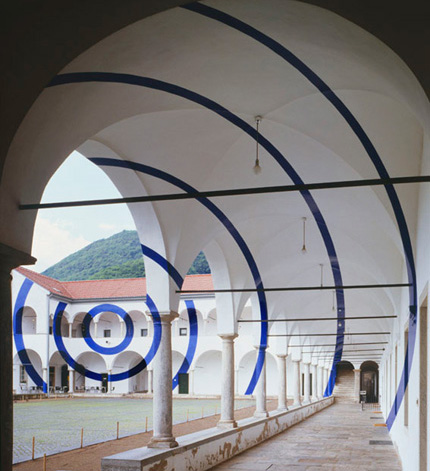
And also:

The photos show that there can easily be two completely different 3D images resulting in the same 2D projection. That said, in most usual scenarios your brain correctly guesses the 3D structure of things based on insufficient 2D inputs. It is important to say that your brain uses a lot of apriori information when reconstructing such scenes. In the absence of such apriori information (as is the case with our 4D cube) our brain’s work is indeed much harder.

Ok, so now that we understand some of the properties of 4D cubes and how projections work, let’s get to the cool stuff – render some 4D images!

The Program

If you are not interested in an implementation of all of the above, you are welcome to skip this section.

I implemented the projection reduction method with a few lines of Python. My program displays an arbitrary shape (box, ring, spiral) of arbitrary dimensions in a universe of arbitrary dimensions (of course dim(universe) ≥ dim(object)!).

The objects are rotated in real time. A color encoding of the high coordinates is also used.

At this point I should add that I wrote this program quite a while ago and for internal use only (i.e. I never thought someone else would look at it – I am actually quite surprised that I even found it and that is still works! [unattended code tends to rot]). I did spend a few minutes in order to enable you to run the program from the command line (instead of from a Python shell), but in order to access all of the options a shell is still required. Also, the code was not at all tested, and running it with the wrong arguments can cause it to throw some exceptions. It is very short though, and all of you with basic python knowledge are welcome to browse it.

A very important part of the code consists of the create_cube and gen_line_pairs functions, defined as follows:

def create_cube(dim=4):
    if dim == 1:
        return [[-1], [1]]
    else:
        res = []
        r1 = create_cube(dim - 1)
        for i in r1:
            res += [i + [-1]]
            res += [i + [1]]
        return res

def gen_line_pairs(rect, dist=1):
    res = []
    for i in range(len(rect)):
        for j in range(i):
            dif = count_dif(rect[i], rect[j])
            if dif <= dist:
                res.append((i, j))
    return res

Can you figure out how they work? :-)

Note that in order to run the program, you will need Python, as well as the Pygame package (which I use for drawing and managing user input). You can try running the program with the following arguments:

> 4d.py 4 rect 4d auto normalize

Some keys you can try:

• Up, down, left, right, home, pageup, return, space, end, pagedown - manually rotating the object (around the four first axes). This only works when automatic rotation is off.
• r – toggles automatic rotation mode.
• 4 – toggles the high-dimensions mode of the automatic rotation. When the automatic rotation is enabled, the object will be rotated around a random axis. When the high-dimensions mode is turned off, the rotation will only take place around the first 3 coordinates. This mode allows appreciating a 3D slice of a high dimension object.
• c – change the coordinate that is used for the color-encoding.

The complete source of the 4D renderer can be found here.

Results

To give all of you without access to python a taste of how some basic primitives do look like in higher dimensions I attached these images. I must say that viewing the objects in motion is much more insightful. I really recommend running the program!

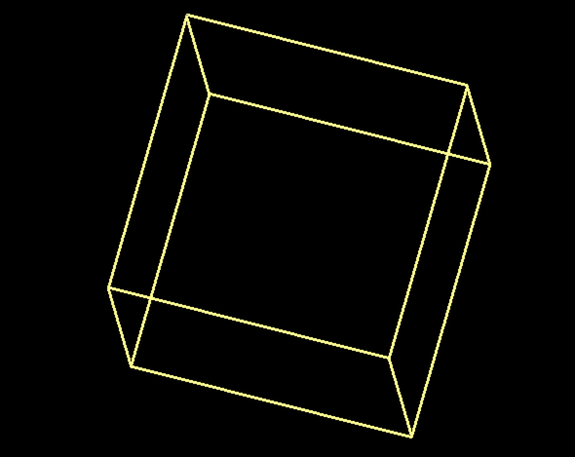
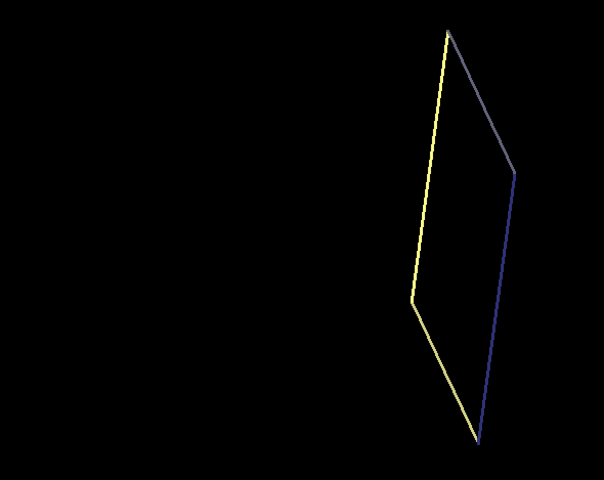
This image shows a regular 3D cube, residing in a 4D universe (after it was rotated a little about all of its axes):

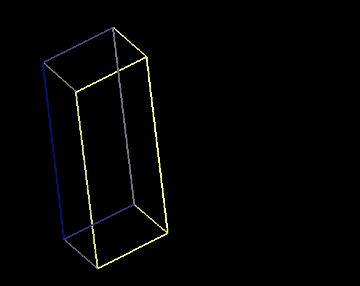
Notice that this is indeed a cube (all its sides are equal!) the reason it appears to be a rectangular box is because the rotation about the 4th axis deforms it. A simpler to grasp, but similar phenomenon occurs while residing a 2 dimensional square inside a 3D universe. After some rotations it may look like this:

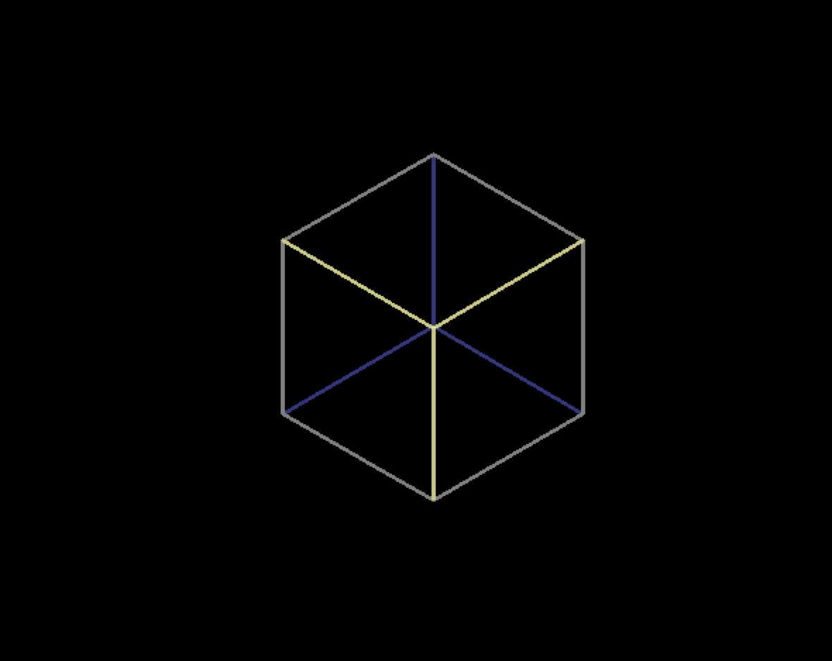
This image shows a 4 dimensional cube:

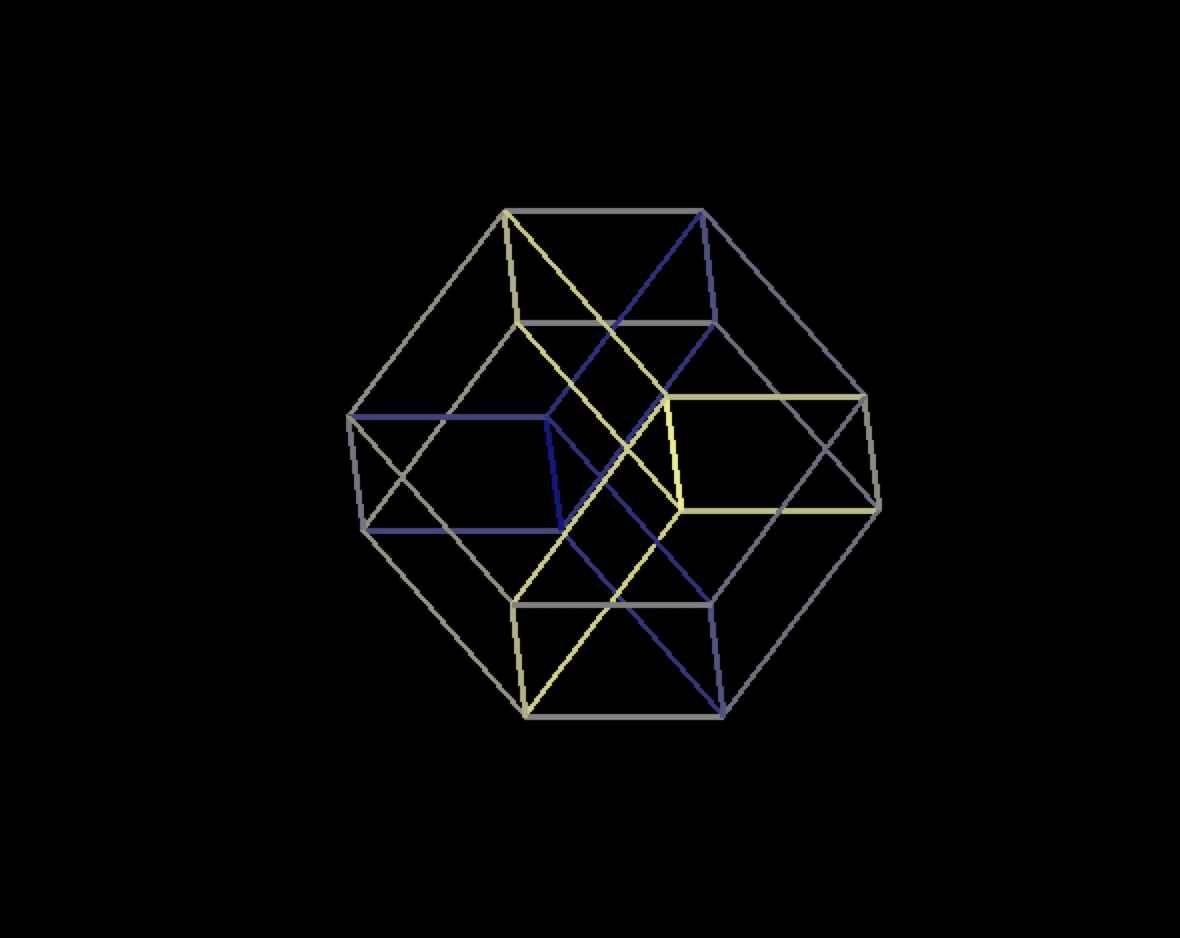
This is perhaps the most interesting object (maybe I will add some more pictures of it).

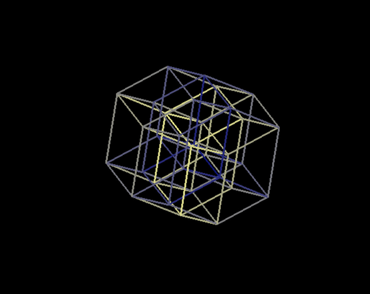
The same cube, this time viewed from a different angle and having its faces interconnected:

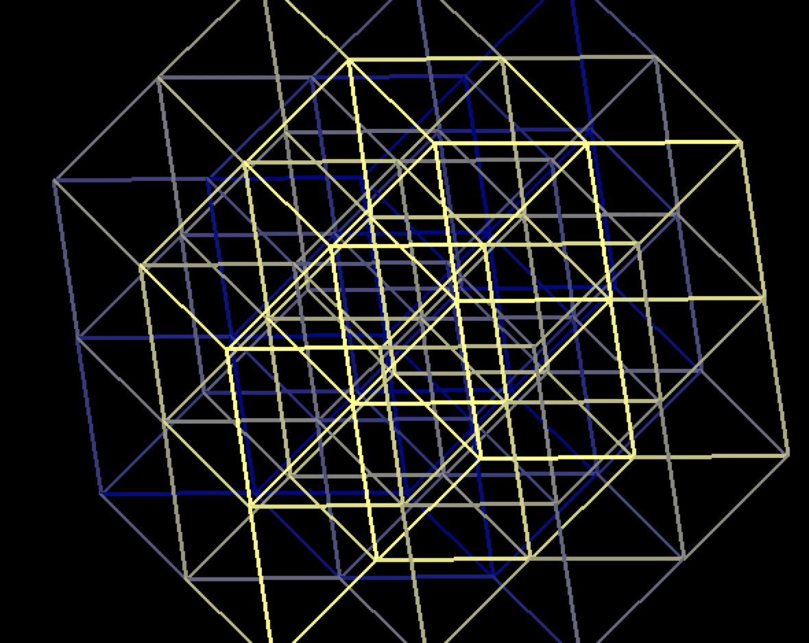
A 5D cube:

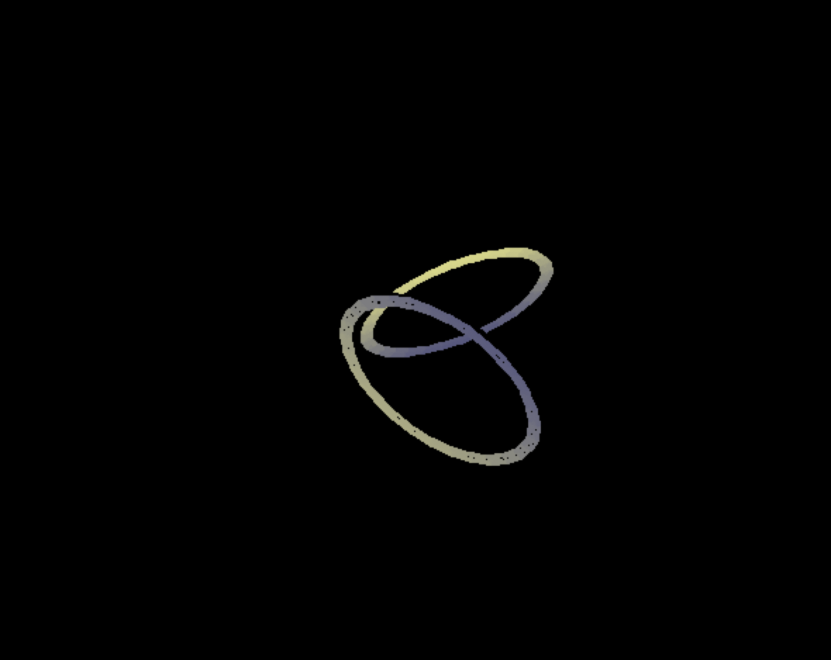
Two rings in a 4D universe:

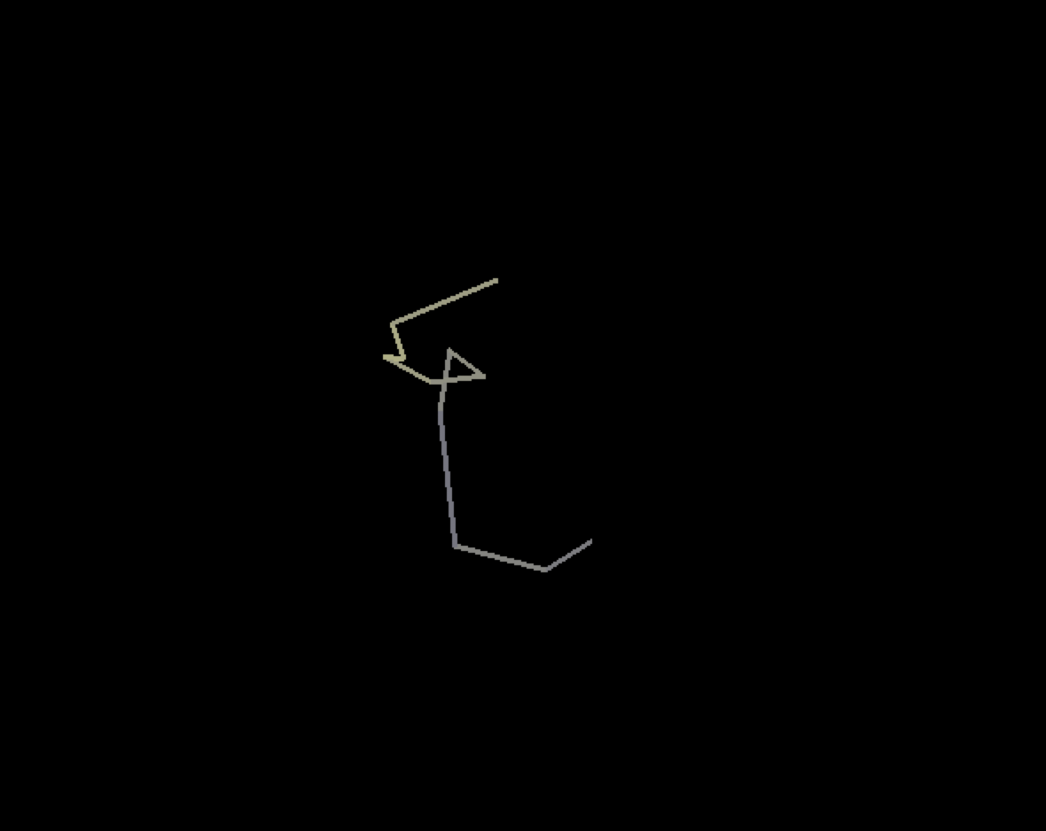
And finally, a very simple 10D spiral in a 10D universe (notice that all the lines are perpendicular!):

Again, these images are much more intuitive when the complete animation is viewed, so download the program and run it!

Enjoy!